Modification and analysis

This type of simulation runs kind of slow. Let's start to use optimization flags (-O) when you compile programs. When compiler is translating the source code to object code, there are many ways to translate the same source code. Compiler analyze the source code, and it will try to make the fastest object code automatically (optimization).

gcc -O3 source.c

There are several levels of optimization (-O1 -O2 -O3). Higher number after -O means more optimization (potentially faster). By default, gcc doesn't do any optimization (equivalent to -O0, 'Oh Zero').

You can see how the optimization influence the speed by

time ./a.out

• Make a function int CntMember(int arr[], int arrSize, int member), which count the occurence of member in an array arr of size arrSize and return the count.

• Use this CntMember() function to check the state of the population every time after the next generation is created. You can count the occurence of ``1'' and if the count becomes 0 or total number of alleles in the population, the extinction or fixation of the allele occured.

• Modify the code, so that it will run the simulations many times (say 1000 replications), and confirm that the fixation probability is equal to the initial frequencies.

• Now you want to collect data of how many generations the two alleles will remain segregating (i.e. time to loss or fixation of 1 allele). Modify the source code to get this data.

  Given the initial frequency of p, the average time to loss or fixation can be approximated by
  

  $$E[T] = - 4 N [ p \cdot ln(p) + (1-p) \cdot ln(1-p) ]$$
  
  
  Kimura and Ohta (1969, Genetics 61:763) used diffusion approximation. Compare your simulation results with this approximation
  

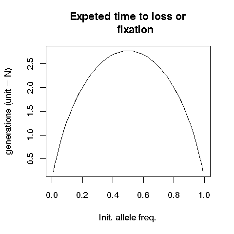
  It remains segregating for the longest time when the initial frequency of an allele is 1/2. This is approximately 2.77 N generations.

• Consider that the population array represents the spatial positions of a linear population (like plants growing along a road). Previously, we assumed that the population is randomly mating, but dispersion may be limited in real populations (``viscous'' populations). Modify the program to incorporate the limited dispersal. Some parameter(s) should be controlling the ``viscosity'' (dispersal distance), and see how these parameters influence the time to fixation or loss. You can make a function CreateNextGenViscous().

• Selection vs drift
  1. We simulated a haploid population. Can you convert the simulation to diploid case? You can cosider that 2 neighboring alleles in the population array is a genotype of one diploid individual. In other words, popB[0] and popB[1] are the two alleles of the individual 1, and popB[2] and popB[3] are the two alleles of the individual 2.
  2. Let's make that the two alleles are under selection. Fitness of genotypes are:
     

     genotype	0 0	0 1	1 1
     fitness	1	1 + h s	1 + s

     s is selection coefficient, h is dominance coefficient.

     For example, you can consider that one beneficial mutant (allele 1) arose in the population (so the rest of the alelles are 0). Even if the advantage of mutation is big, it will get lost most of the time. You can check how the probability of ultimate fixation of allele 1 is influenced by dominance.

• Other modification exercises:
  
  • You can create two (or more) populations: each population can be represented by an array. You can easily simulate gene flow between the populations. Example, when you are creating the next generation, you can draw a uniform random number [0,1) and if it is less than probability of migration m, you can draw the gamete from the other population(s).
  • Instead of 2 alleles, you can have many alleles like microsatelites. You can assume some mutational models (e.g, allele 6 can only mutate to allele 5 or allele 7 etc).