Quick tour of R

In this section, we'll look what kind of things R can do. I'll save the detail for the later section.

Let's say that we had grew 10 plants in shady and sunny environments, and measured the leaf lengths and width. You can use the data imported in the previous Exercise. If you didn't do the importing exercise, here is the converted text file.

• Read in a tab delimited file, and create a data frame.

  dat.in <- read.table("data.txt", header=T, sep="\t")
  

• Check the contents.

  names(dat.in)
  dim(dat.in)
  dat.in
  

• Some data exploration
  1. Scatter plot

     plot(dat.in$leaf.len, dat.in$leaf.width)
     

     
     This shows the leaf length and width seems to be correlated.

  2. Calculating the correlation, ``use='' option specify how to deal with NA's.

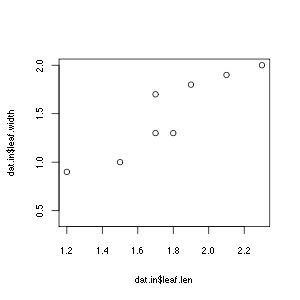
     cor(dat.in$leaf.width, dat.in$leaf.len, use="complete.obs")
     

  3. box plot

     boxplot(leaf.width ~ treatment, data=dat.in)
     

     
     This shows the plants in sunny environment have bigger leaves.

  4. Mean leaf width for each treatment group: 0.98 for shade and 1.86 for sunny.

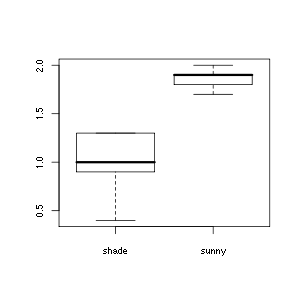
     mean(dat.in[dat.in$treatment == 'shade', "leaf.width"])
     mean(dat.in[dat.in$treatment == 'sunny', "leaf.width"])
     

  5. linear model (ANOVA)

     anova.fit <- lm (leaf.width ~ treatment, data=dat.in)
     anova(anova.fit)
     

     Created anova table:

     Analysis of Variance Table
     
     Response: leaf.width
               Df Sum Sq Mean Sq F value    Pr(>F)    
     treatment  1  1.936   1.936  25.813 0.0009523 ***
     Residuals  8  0.600   0.075                      
     ---
     Signif. codes:  0 '***' 0.001 '**' 0.01 '*' 0.05 '.' 0.1 ' ' 1
     

     Slightly differnt wayt to look at the fit of linear model.

     summary(anova.fit)
     

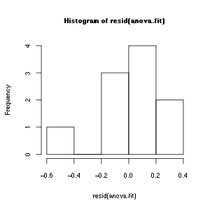
     Looking at the distribution of residuals:

     hist(resid(anova.fit))
     

     
     This doesn't make a nice gaussian distribution because there are only 10 observations.

Exercise: repeat the analysis with leaf.len (start from producing the box plot).